This post describes the vector graphics renderer of Orca. For previous posts about my exploration of different vector graphics rendering techniques, you can see this series.

Introduction

Orca provides a canvas API out of the box, which allows apps to draw 2D vector graphics, and also powers the rendering of the UI system. Users can build paths from line segments and Bézier curves, and fill or stroke paths using a number of attributes such as the path color, gradient, texture, line width, etc.

Here is an example of what some simple drawing code might look like:

// background
oc_set_color_rgba(0, 1, 1, 1);
oc_clear();

// head
oc_set_color_rgba(1, 1, 0, 1);
oc_circle_fill(x, y, 200);

// smile
oc_set_color_rgba(0, 0, 0, 1);
oc_set_width(20);
oc_move_to(x - 100, y + 100);
oc_cubic_to(x - 50, y + 150, x + 50, y + 150, x + 100, y + 100);
oc_stroke();

// eyes
oc_ellipse_fill(x - 70, y - 50, 30, 50);
oc_ellipse_fill(x + 70, y - 50, 30, 50);

And here is the image it produces:

The API is implemented by a WebGPU compute backend which is, at its core, similar to traditional software rasterizers, but uses a couple tricks to efficiently split and parallelize the workload on the GPU. Its rendering method is based on (Nehab and Hoppe 2008) and (Ganacim et al. 2014). Raph Levien’s blog posts such as this one and this one were also a great resource and inspiration.

Winding Numbers and Fill rules

For each pixel, and each shape, the renderer has to decide if the pixel is inside or outside the shape, and shade it accordingly.

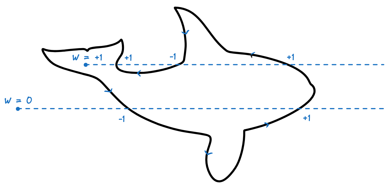
For a given pixel and a given shape, we can consider a horizontal ray going from the pixel to the infinity on the right, and count the signed intersections between the ray and the shape’s oriented contour (Figure 1):

• We count +1 when the ray crosses an edge going up.
• We count -1 when the ray crosses an edge going down.

This count is called the winding number of the pixel with respect to that shape.

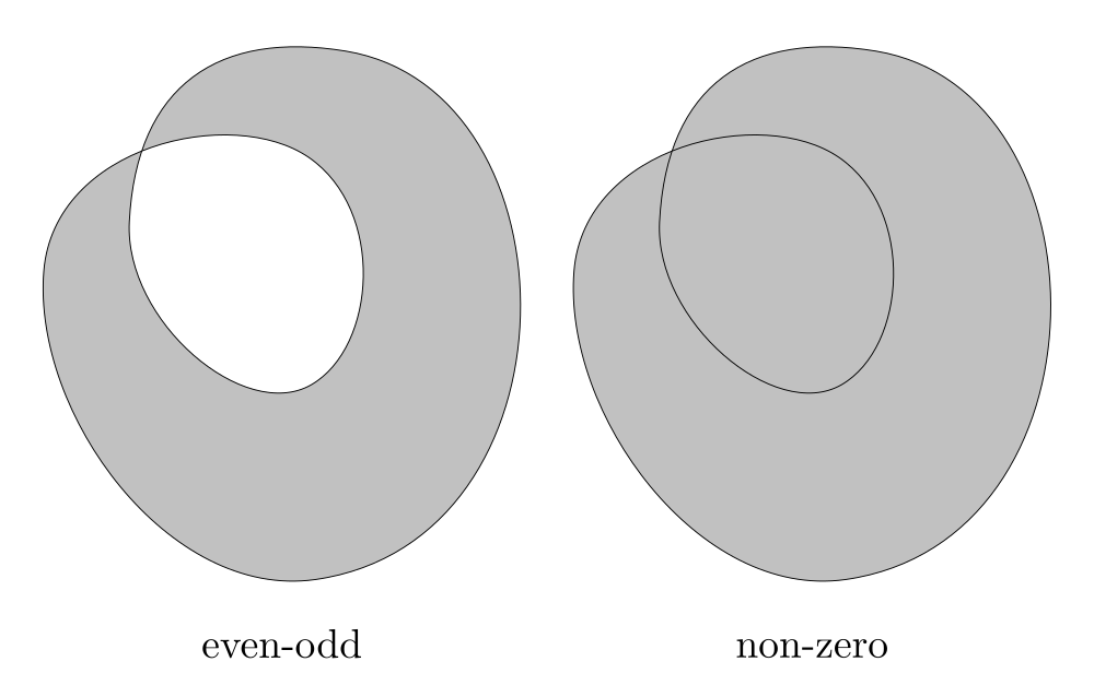
We can then choose a fill rule to decide if the point is inside the shape:

• With the even-odd rule, the point is considered inside the shape if the winding number is even, and outside otherwise.
• With the non-zero rule, the point is considered inside the shape if the winding number is non zero.

In simple cases these rules produce the same result, but they differ in how they handle shapes with holes or self-intersecting shapes (Figure 2).

Winding Numbers Computation

Let’s suppose we have a path \(P\) that is defined by a set of line segments, and quadratic and cubic Bézier curves. Intersecting our scanlines directly with these curves can be pretty difficult, so in order to simplify the computation of winding numbers, we can first split them into monotonic curve segments (ie segments that go either right or left and either up or down, but never “curve back”). Line segments are already monotonic. Splitting quadratic and cubics into monotonic segments first requires finding the split points by solving a couple linear and quadratic equations, as explained in (Ganacim et al. 2014). Bézier curves can then be split at those points using blossoms.

Now that we have monotonic curves, we can classify them into one of four possible configurations, namely top-left (TL), top-right (TR), bottom-left (BL) and bottom-right (BR), depending on which corner of its bounding box the curve bends towards (Figure 3).

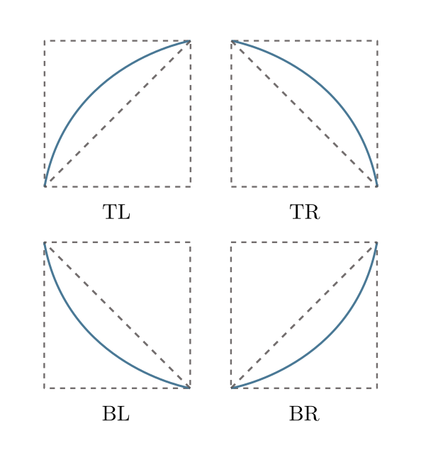
For the computation of winding numbers we also need to know if the segment is going up or down. By convention, we consider line segments as being either BR or TR, horizontal segments as going up, and vertical segments as going right.

We can then check a pixel against a curve segment by sequentially applying the following rules:

• If the pixel is above, below, or to the right of the segment’s bounding box, the scanline doesn’t intersect that segment.
• If the pixel is to the left of the segment’s bounding box, the scanline intersects the segment.
• If the segment is BR or TR and the pixel is to the left of the endpoints’ diagonal, the scanline intersects the segment.
• If the segment is TL or BL and the pixel is to the right of the endpoints’ diagonal, the scanline doesn’t intersect the segment.
• Otherwise, the scanline intersects the segment if the pixel is to the left of the segment.

All these tests but the last are a few checks against a bounding box or a line. Only the last case requires a test against the actual curve to know on which side the pixel lies.

This can be done by transforming our parametric curve into an implicit curve equation, as described in (Loop and Blinn 2005). In short, we can compute a sign \(s\) and a matrix \(K\) that transforms a point’s homogeneous coordinates \((x, y, 1)\) to coordinates \((k, l, m)\) such that the space on the left of the curve is defined by Equation 1 : \[ \begin{cases} (k^2-l)m < 0\,, \; &\textrm{for quadratic Béziers} \\[6pt] s(k^3-lm) < 0\,, \; & \textrm{for cubic Béziers} \end{cases} \](1)

The implicit equation matrix \(K\) and sign \(s\) can be baked into each segment. Checking on which side of the curve a point lies can then be done by multiplying that point by the matrix, and evaluating the equation with the resulting coordinates.

Tiling

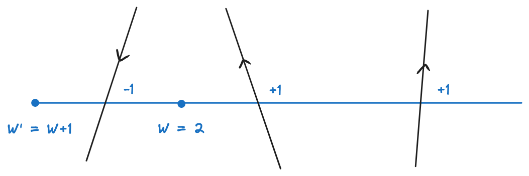
If we were computing the winding number for each pixel independently, we would do a lot of redundant work. A pixel \(P_1\) shares most of the computation with its right neighbor \(P_2\), since its winding number is equal to that of \(P_2\) plus the number of signed crossings between \(P_1\) and \(P_2\) (Figure 4). The winding numbers of pixels on the same scanline can thus be computed with a prefix sum of signed crossings along the scanline, from right to left.

This is a little bit better, but we would still need to check each shape with each scanline. We would also still do a lot of redundant work because most of the time, the winding number for a pixel shares computations not only with the pixels on its right, but with other pixels in a close neighborhood.

Lattice Clipping Algorithm

Ideally, we would like to partition the whole canvas into such small neighborhoods, like square tiles, and compute the winding numbers of the pixels in each tile independently, only taking into accounts edges that overlap that tile. This is not possible because as we just saw computing the winding number of a pixel is not a local problem: it depends on intersections happening far to the right of this pixel. However, using a lattice clipping method exposed in (Nehab and Hoppe 2008), we can split the problem into a local one and a non-local one. The first problem can be solved independently for each tile. The second problem still requires a prefix sum, but along a row of tiles, not pixels.

Shortcuts Segments

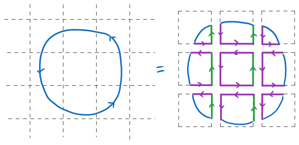
Lets consider a path \(\mathcal{P}\) spanning multiple tiles of a regular grid. In each tile \(\mathcal{T}\), we can build an equivalent path (one which produces the same winding numbers for all pixels \(\mathcal{T}\)), by keeping the segments of \(\mathcal{P}\) that overlap \(\mathcal{T}\) and adding shortcut segments along the edges of the tile Figure 5. In practice shortcut segments on the left, top, and bottom of the tiles (shown in purple) can be ignored, since they don’t participate in the computation of the winding number.

Of course we don’t know, just looking at a single tile, if the shortcut segments we add on the right edge should go up or down. However, the clever idea of the lattice clipping method is that we can make a consistent guess, and correct it afterwards.

Local Shortcuts and Backdrop

Since the path is closed, a segment that leaves the tile from the right edge must either reenter the tile from the right edge, or exit the row of tiles, from the top or the bottom. Figure 6 shows the three configurations.

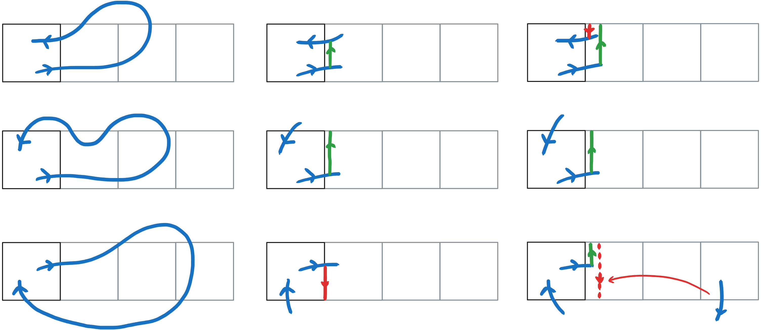
The left column shows and example path exiting and returning to the tile. The middle column shows the shortcut segments we would need to insert to create an equivalent path in the tile, but that we can not determine locally. Instead, on the third column, we make a guess that these shortcut segment should join the exit (resp. entry) point at the right edge and the top of the row, going up (resp. down).

• For case 1, it works because shortcut segments both add and cancel out to create the equivalent of the shortcut segment in the middle column.
• Case 2 is identical as the middle column.
• In case 3, we are making a wrong guess, but we can correct it afterwards. When we encounter a path segment that crosses a tile’s bottom boundary, we know that all tiles on the left wrongly assumed that it would exit from the top. So we can correct them by adding a backdrop segment, i.e. adding \(+1\) to the winding numbers of all their pixels if the crossing path is going up, or \(-1\) if it is going down.

NOTE 1: Since we have monotonized curve segments, we don’t need to exactly compute the intersections of segments width the right edge. It is equivalent to add a shortcut segment going from the end point of the curve outside the tile to the top of the row (or no shortcut if the segment exits the row from above).

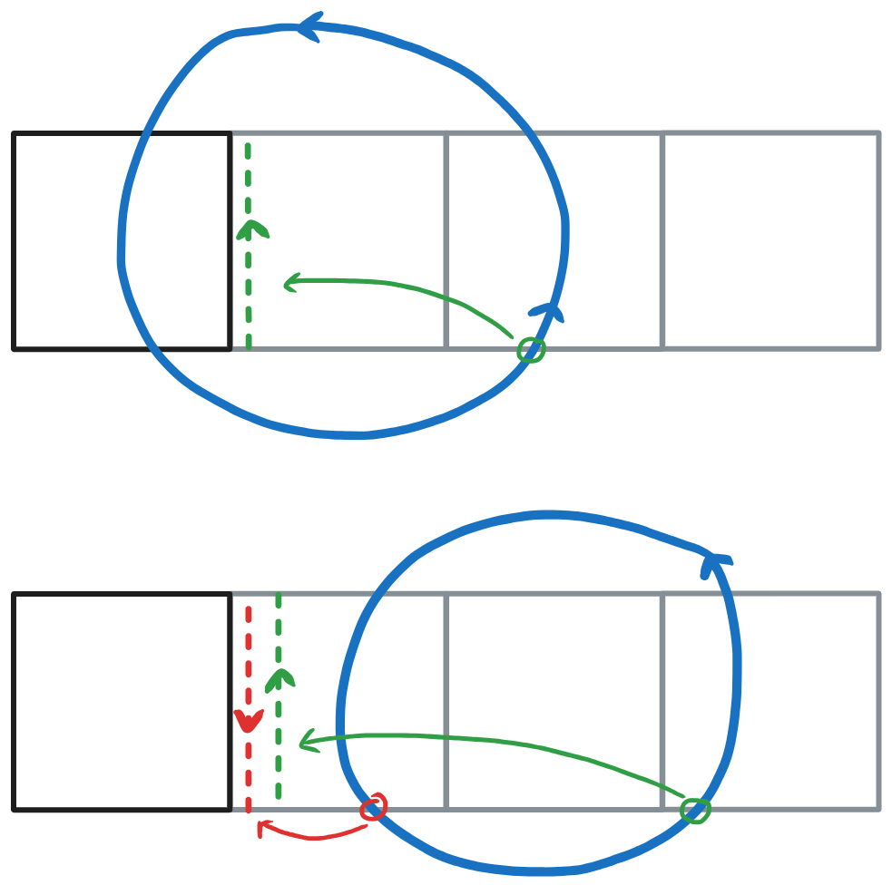
NOTE 2: For tiles that do not have a path segment exiting from the right, we don’t have to create shortcut segments at all: the winding numbers are corrected by the same mechanism as for case 3 (Figure 7).

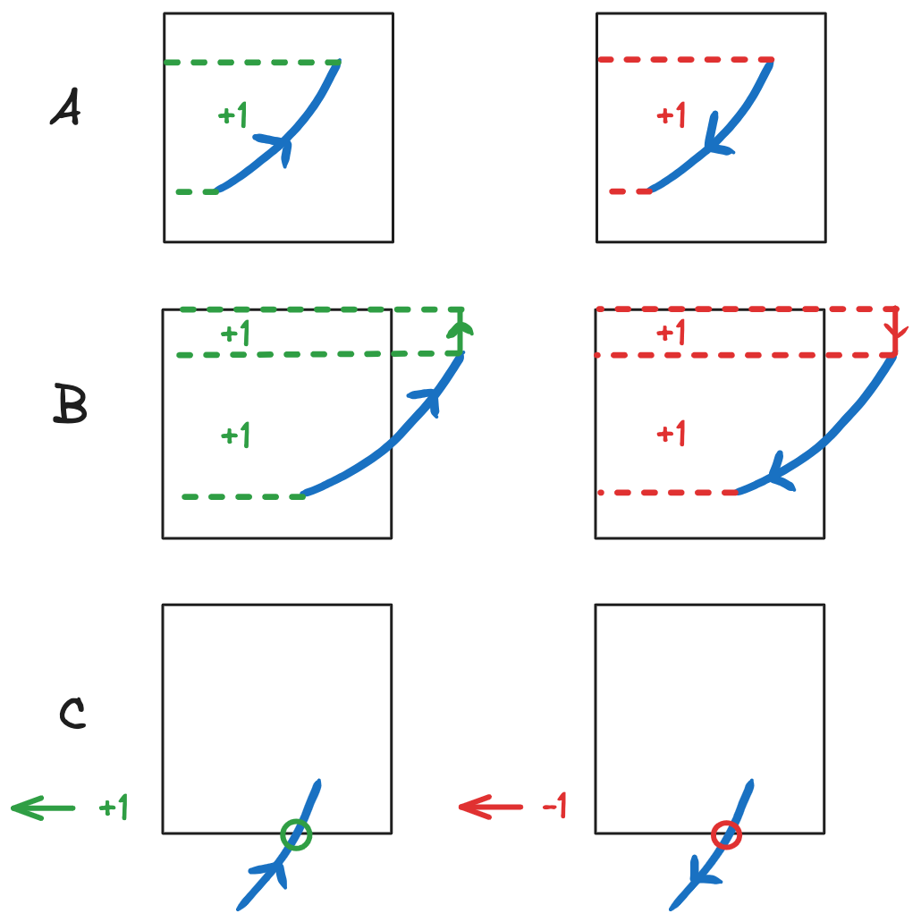
Finally, we can state three rules to locally compute the winding numbers of cells (Figure 8):

• For a segment going up (resp. down) add \(+1\) (resp. \(-1\)) to the winding numbers of pixels to its left (case A, B, and C).

• If a segment exits (resp. enters) through a right boundary, add \(+1\) (resp. \(-1\)) to the winding numbers of pixels above the outside endpoint of the segment (case B).

• If a segment going up (resp. down) crosses a bottom boundary, add \(+1\) (resp. \(-1\)) to the winding numbers of pixels in all tiles to its left (case C).

Implementation

With what we’ve seen so far, we can start to sketch out the outlines of a renderer:

• First split paths into monotonic, implicit curve segments.
• Bin segments into tiles. When a segment is crossing the bottom edge of a tile, update the winding offset to be applied to the tiles on the left.
• Compute the prefix sum of winding offsets along tile rows, from right to left.
• For each tile independently, and each pixel within the tile, compute the local winding number and add the tile’s winding offset. Apply the fill-rule to decide whether or not to shade the pixel.

This big picture is somewhat complicated by the fact that we can have multiple overlapping and transluscent paths, which means we also need to take care of the following:

• We need to make sure we compute a separate winding number for each path, taking into account only the curve segments belonging to that path.
• We must process paths in an order that allows correct occlusion and blending.

This seem to require a lot of sequential work and potential overdraw. However there’s a few key insights that can allow us to cull unnecessary work and split the workload to be run more efficiently on the GPU:

• Although we must keep curve segments grouped by path, the order in which we process the segment inside a path doesn’t matter. We can thus bin segments to tiles all in parallel, as long as we keep separate bins for each path.
• We can detect tiles that are entirely filled by a path early on, after doing the prefix sum. These are tiles with no segment, but a non zero (or odd) winding offset. If the fill color for the corresponding path is opaque, we can also avoid processing paths below it in that tile.
• Although we need to maintain sorting between paths when shading pixels, we can use premultiplied alpha to blend them front-to-back. This allows us to stop at the first opaque pixel and avoid unnecessary overdraw.

Orca’s pipeline overview

The renderer’s pipeline is shown Figure 9. Each rounded box represents a compute shader, and blue arrows represents dependencies between those shaders. Dotted arrows point to the data structures these shaders consume or produce. The architecture is similar to, and inpired by the one presented by Raph Levien in this post, although the detail of the data structures and how the workloads are split can differ.

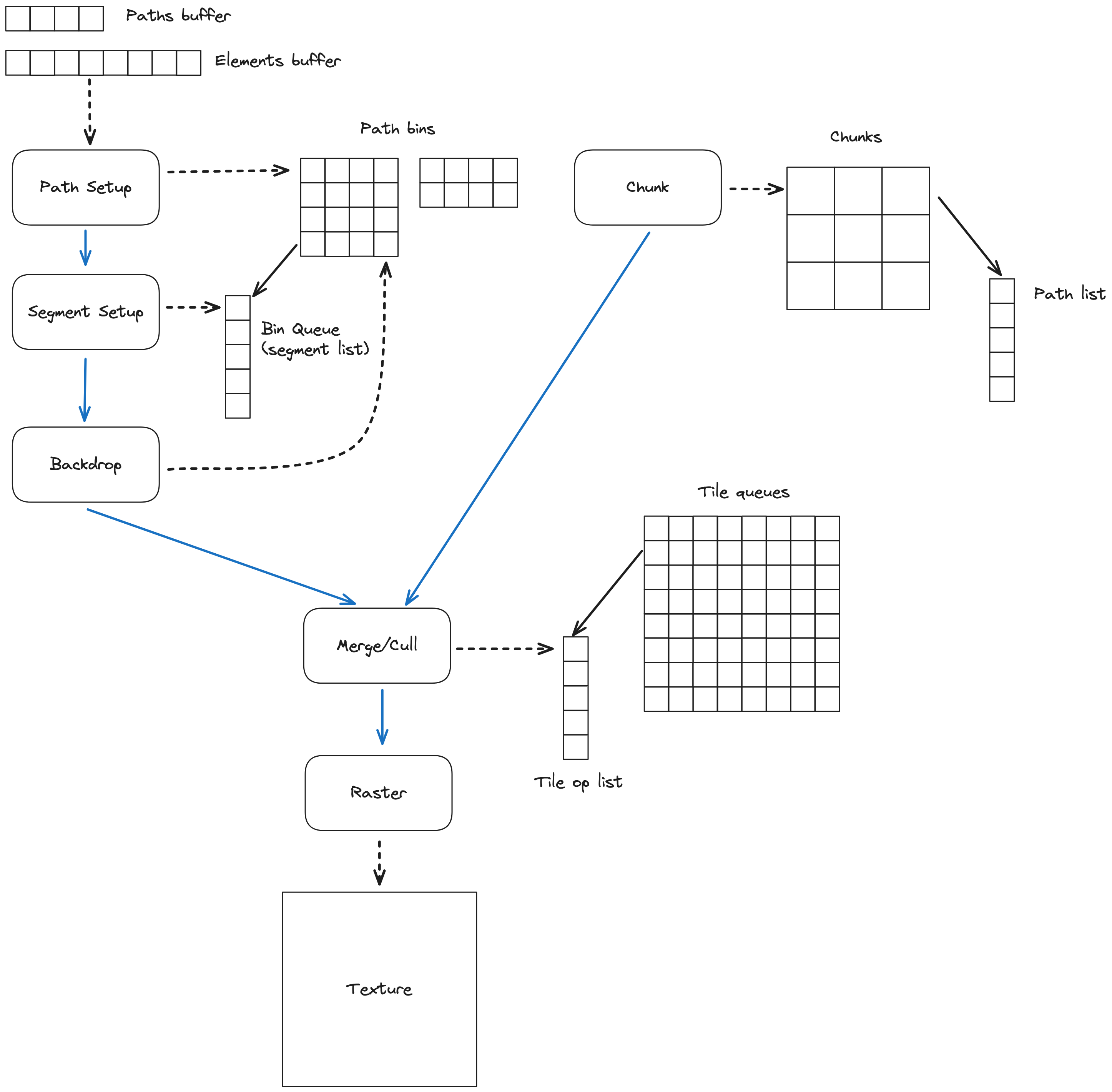
The inputs are a paths buffer and an elements buffer:

• The paths buffer contains attributes for each path, including the path color, gradient, or texture, and the path clipping rectangle.
• A path element can be a line segment, or a quadratic or cubic Bézier curve. It contains the control points of the segment, as well as the index of the path it belongs to.

The screen is partitionned into 16 by 16 pixels tiles. The pipeline builds a list of tile ops for each screen tile. Tile ops can be one of the following:

• OP_FILL unconditionally shades the pixel with a path’s color.
• OP_CLIP_FILL shades the pixel with a path’s color if it is inside the path’s clip rect.
• OP_SEGMENT checks the pixel against a given segment and updates its winding number accordingly.
• OP_END adds a winding offset to the pixel’s winding number, and apply the path’s fill rule to shade the pixel.

The raster pass then traverses the lists of tile ops and applies each operation to shade pixels.

Path Setup: We first dispatch a thread for each path. Each thread allocates a set of bin queues corresponding to the tiles covered by the path’s bounding box. Each bin queue stores a pointer to the head of a linked list of tile ops, as well as a winding offset.

Segment Setup: We dispatch a thread for each path element. Each thread splits its path element into monotonic implicit curve segments, and bins these segments to its path’s bin queues.

For each tile touched by a segment, we create a new OP_SEGMENT tile op and link it in the corresponding bin queue. If the segment crosses the right boundary of the tile, we mark the op accordingly. If the segment crosses the bottom boundary of the tile, we update the winding offset of the bin queue.

Backprop: We dispatch a workgroup of 16 threads per path. Each thread picks a row to process by atomically bumping a workgroup counter, and propagates the winding offsets to the left. Threads continue to pick and process rows until all rows have been processed.

Chunk: This pass is not strictly necessary but it adds a level of tiling that greatly accelerate the next pass. It dispatches one thread per chunk of 16 by 16 tiles. Each thread produces a list of paths that overlap its chunk.

Merge / Cull: This pass merges the tile op lists produced by the segment setup pass to build tile queues. It dispatches one thread per tile. The thread goes through through the path list of its chunk in front-to-back order, and process bin queues that correspond to its tile:

• If the tile is outside the path’s clip, the bin queue is ignored
• If the bin queue has a non-empty tile op list, it is linked into the tile queue, followed by an OP_END tile op.
• If the bin queue is empty but has a non-zero winding offset, the thread inserts an OP_FILL or OP_CLIP_FILL into the tile queue, depending on whether the tile is completely or partially inside the path’s clip.

The process stops after inserting the first OP_FILL with a solid color.

Raster: This pass traverses the tile queues and shades pixels, writing the resulting color to an output texture. It also handles blending and multisample anti-aliasing.

We dispatch one workgroup per tile and one thread per pixel. Each thread maintains a single output color and an array of winding numbers for up to 8 subpixel samples in its pixel. The thread goes through the list of tile ops of its tile, and updates the winding numbers and color accordingly:

• OP_FILL blends the path color with the current color.
• OP_CLIP_FILL computes a coverage value by checking each sample against the path’s clip. It then uses that value to blend the path color with the current color.
• OP_SEGMENT checks each sample against the segment and update their winding numbers.
• OP_END adds the winding offset, and computes a coverage value from the subpixels winding numbers and the fill rule. It then uses that value to blend the path color with the current color.

The current path color can be a single fill color, or can be computed from a gradient or sampled from a texture.

Texture Batching

Due to limitations of WebGPU, we can’t use bindless textures. This means that we can only bind a limited number of source images to the raster shader. If our scene uses more images, we have to break it into batches, and do a separate draw call with different texture bindings for each batch.

This also means we need to blend the results of the raster pass with that of previous batches. The raster pass thus writes to an intermediate texture, and we use a simple render pass to blend that to our output texture. This is possible because premultiplied alpha blending is associative.

At the very end, we use a final render pass to apply gamma correction and blit our output texture to the frame buffer.

Performance

Currently on my 2019 MacBook Pro with an AMD Radeon Pro 5500M GPU, the Ghostscript Tiger Figure 10 renders in a 1600x1200 canvas with 4xMSAA in 10ms. This is still a lot slower than what I expect is achievable with this method, but I haven’t really done any optimizing work yet. Raph Levien has much better numbers even on an integrated Intel GPU, using a very similar method, so I’m hopeful there’s a lot of room for improvement.

I plan on doing a more thorough assessment of performance and improve the renderer later on, after tackling some higher-priority tasks. In the meantime, it is already “good enough” to start using with our UI system and draw simple to moderately complex scenes.

Conclusion

This is the end of our tour of the Orca vector graphics backend. I hope you enjoyed it! As always, I’m happy hearing feedback and answering questions in the Handmade Netwok Discord. If you liked this post and want to support my work, please consider donating through Github Sponsor or my Donorbox form. This will help me work on Orca and write more of these technical posts along the way.

Take care, and see you~

References